The next two lessons will focus on techniques which involve reshaping waveforms by modulating a simple (often sinusoidal) waveform. These modulation techniques include:
- Ring Modulation (aka Balanced Modulation, Amplitude Modulation)
- Waveshaping
- Frequency Modulation
- Phase Distortion
Each type of modulation creates a new waveform that has more harmonic content than the original. The modulating oscillator (or modulator) is connected to either the frequency or amplitude of the audible oscillator (or carrier). Varying the amplitude or frequency changes the slope of the carrier waveform continuously, and this creates new harmonics in the resultant waveform. These new harmonics are called sidebands, as they appear on both “sides” of the carrier frequency – both lower and higher.
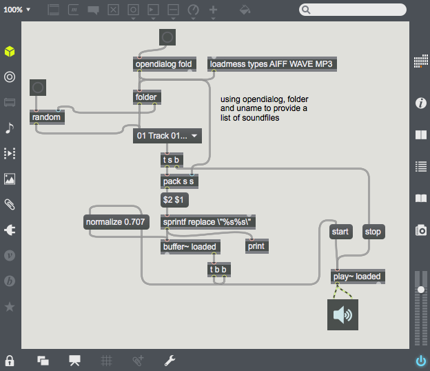
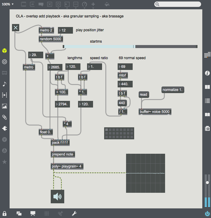
Patches for this week are located here: w4rmwsenv. In this case, these patches are starting points – the techniques are developed further in this post. Also included are some simple examples of mixing and envelope usage.
Ring Modulation
This technique is called ring modulation because of the ring of diodes used in the analog implementation of this technique.
Digitally, the technique is much simpler, one simply needs to multiply the amplitude of the carrier oscillator by the output of the modulating oscillator. Here is a simple example:
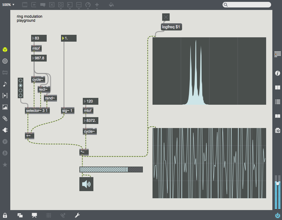
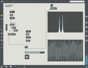 The carrier is at a fairly high frequency (8372 Hz), and the modulator is at 987.8 Hz. Note that the output consists of two harmonics – one is at C – M (~7384) and the other at C + M (~9360 Hz). These two sidebands are created by the sum and difference of the slopes of the two oscillators. The carrier oscillator is completely absent (this is referred to as “carrier suppression”). One can bring back the carrier by adding an offset to the modulating waveform as in the following patch:
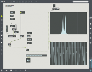
Here a signal of value 1.0 is added to the modulating waveform. This signal is multiplied by the carrier. The carrier then appears in the sonogram in the middle of the two sidebands.
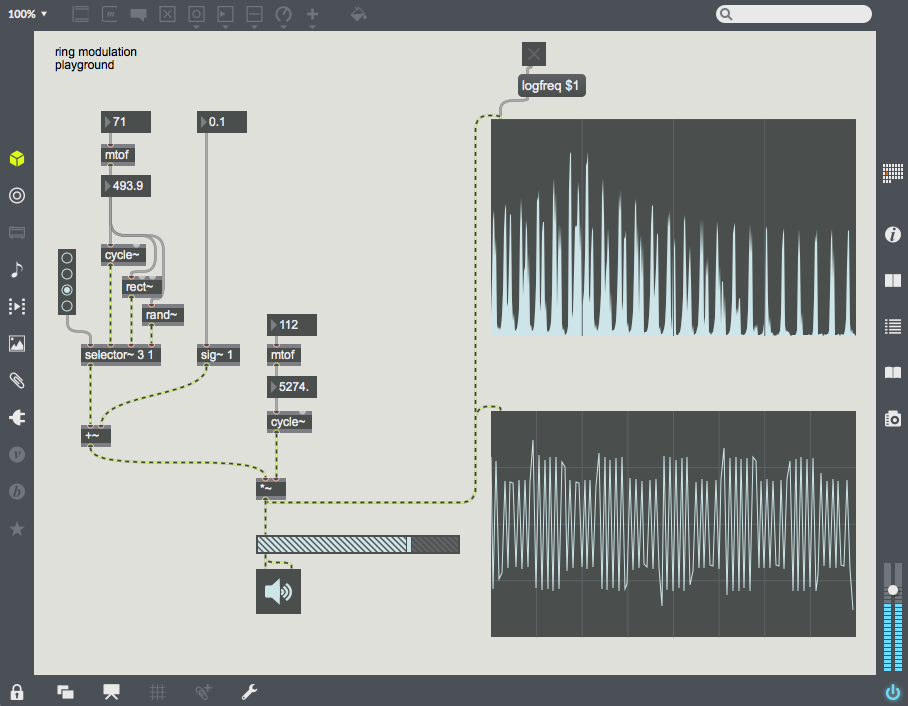
Different signals can be used for the carrier or modulator. In this patch a radio button and selector~ object is used to change the modulator waveform. All the harmonics of the  modulator are now applied to the carrier, giving a much denser waveform. For example, choose the 3rd radio button to use a square waveform. Here one can see all of the harmonics of the square wave on either side of the carrier. Also notice that low sideband harmonics wrap-around 0 Hz, and proceed back upward.
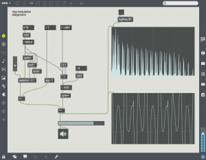
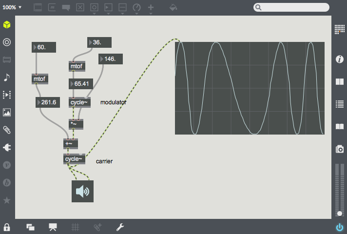
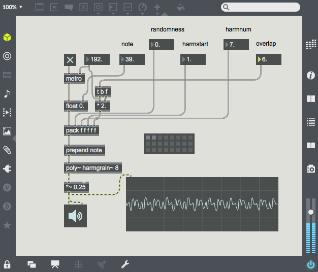
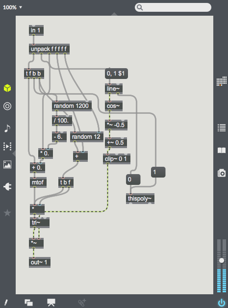
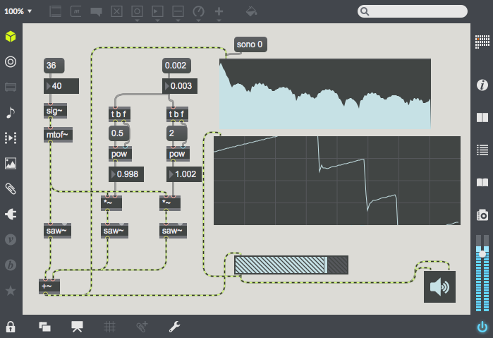
Most of the time, ring modulation creates rather dissonant or non-harmonic timbres. This can be limited by relating the frequencies of the carrier and modulator by integers or simple ratios. In this example the carrier is 5/3 the frequency of the modulator.
Single Sideband Ring Modulation (AKA Frequency Shifting)
With a little more effort the upper or lower sideband from ring modulation can be suppressed. This technique requires a sine and cosine oscillator pair for the modulating oscillator, and a 90 degree phase shifted version of the carrier.
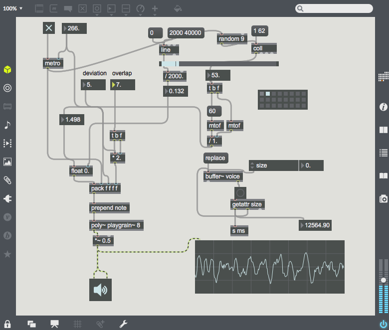
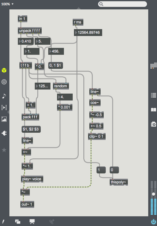
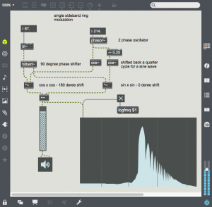 A multiply of sin x sin and cos x cos will create a 180 degree and 0 degree phase shifted components. Adding the two products will leave only the upper sideband. In Max one can use the hilbert~ object to create sin and cos components from any sound source. In this example, a triangle wave is being processed by hilbert~. The frequency of the modulator is the frequency shift of the upper sideband. As the triangle wave is shifted upward, you can hear the harmonics go out of tune, One can also apply SSB ring-modulation/frequency shifting to sound files or live sound sources. At small settings there is still some harmonic integrity, but this soon disappears.
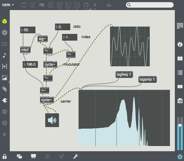
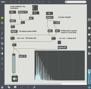 Another variant of this technique is to use feedback to create a series of harmonics. If the carrier and modulator are related by simple ratios, a consonant timbre is created. Also, as feedback is increased – the gain is increased, so output volume may need to be adjusted to avoid clipping distortion
Wave Shaping
And speaking of clipping distortion, another form of amplitude processing is wave shaping, a technique in which the original waveform is reshaped by a transfer function. The function is used to map input values to output values and will change the harmonic content of the original waveform.
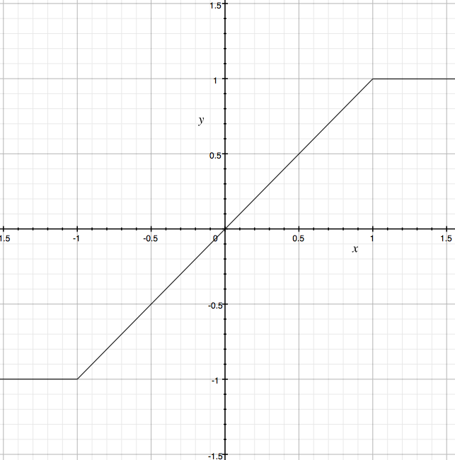
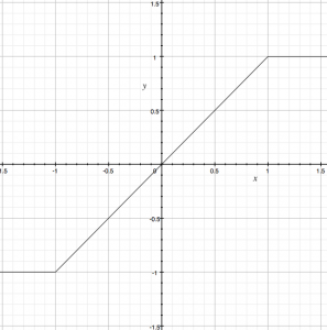 A very typical transfer function is one which produces clipping when the input reaches a limit. In this transfer function, the input value is mapped to the x-axis, and the output on the y-axis. One can think of the input coming in the bottom of the function and the output proceeding out of the right of the function. You can see that when the input goes above 1.0, the output is clipped to 1.0, and similarly the output is clipped to -1.0 for input signals below -1.0. This transfer function is similar to simple amplifier distortion, much like what you would find in a two transistor fuzz pedal. The clipping in this case will add a great number of harmonics to the input signal (aka harmonic distortion). Also note that a steeper slope will produce gain equivalent to the slope.
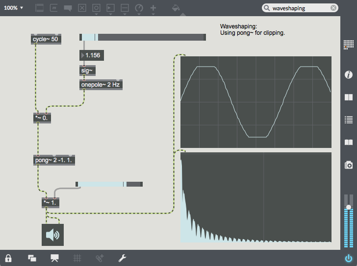
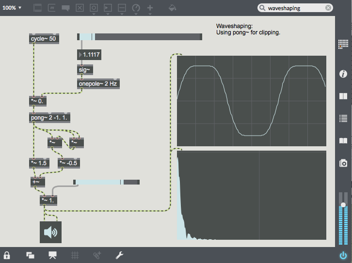
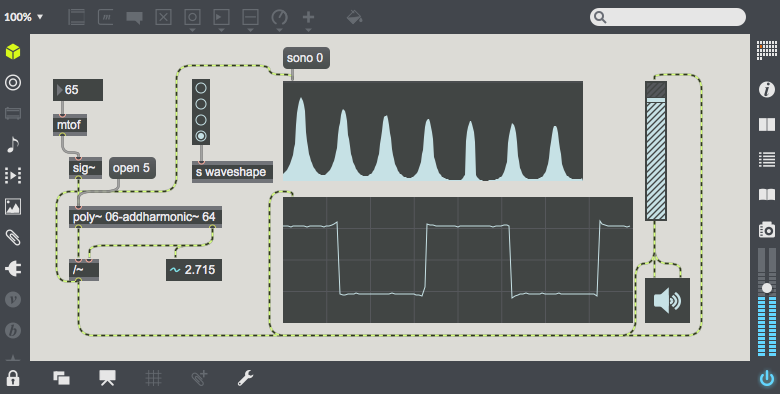
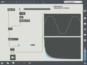 This transfer function can be implemented in Max with a multiply for the slope between -1.0 and 1.0 and by using pong~ to limit the wave to -1.0 and 1.0. in this case the sine wave is shaped into a sine with the top and bottom flattened. The spectrogram shows the additional harmonics added by this clipping.
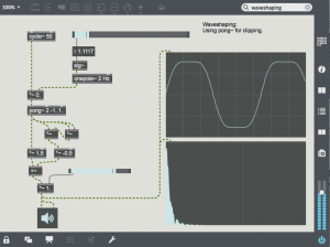 The polynomial “y = 1.5 * x – 0.5 * x^3” can be added to this waveshaper to soften the transition to a clipped waveform. This polynomial causes the slope to decrease as x increases. Any polynomial can be used in Max as a waveshaping function. In this example the polynomial is inserted after the clipping function as the x^3 term will increase rapidly after x passes the -1.0, 1.0 limit.
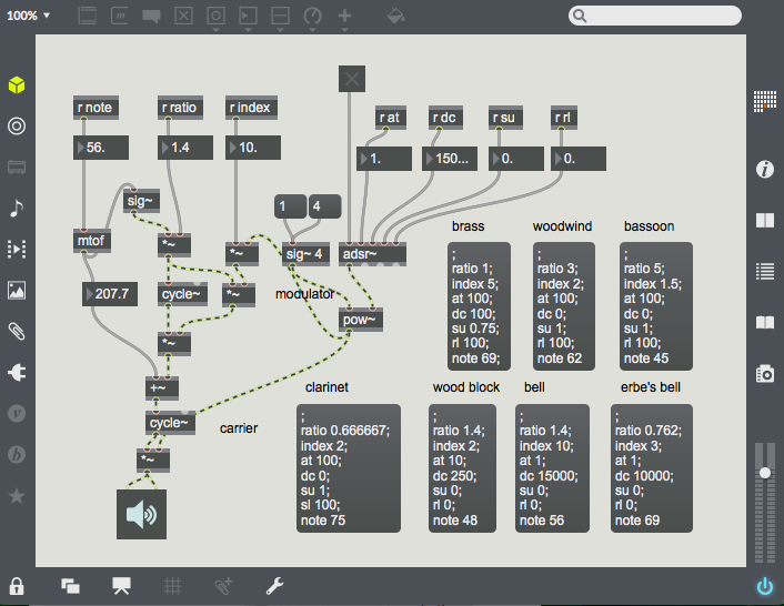
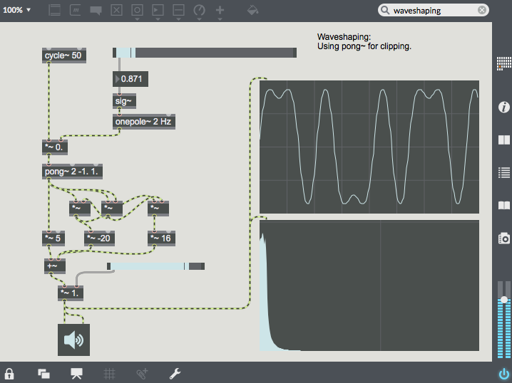
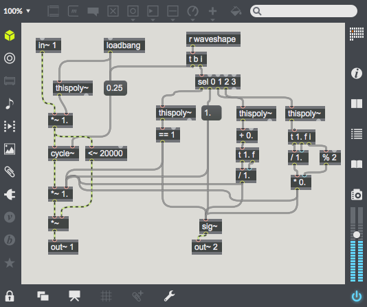
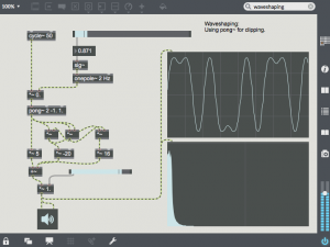 Chebyshev polynomials are also often used for waveshaping as they can transform a sine wave into it’s harmonic. This example uses the 5th chebyshev polynomial “y=16x^5 – 20x^3 + 5x. As gain increases from 0.0 to 1.0, the output is reshaped from the fundamental to the 3rd partial to the 5th partial. Multiple chebyshev polynomials can be combined. This type of waveshaping can be very useful when creating tones which have more harmonic content as the amplitude increases.
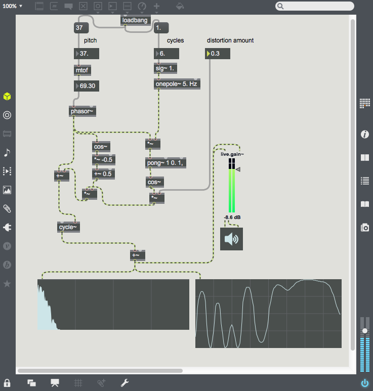
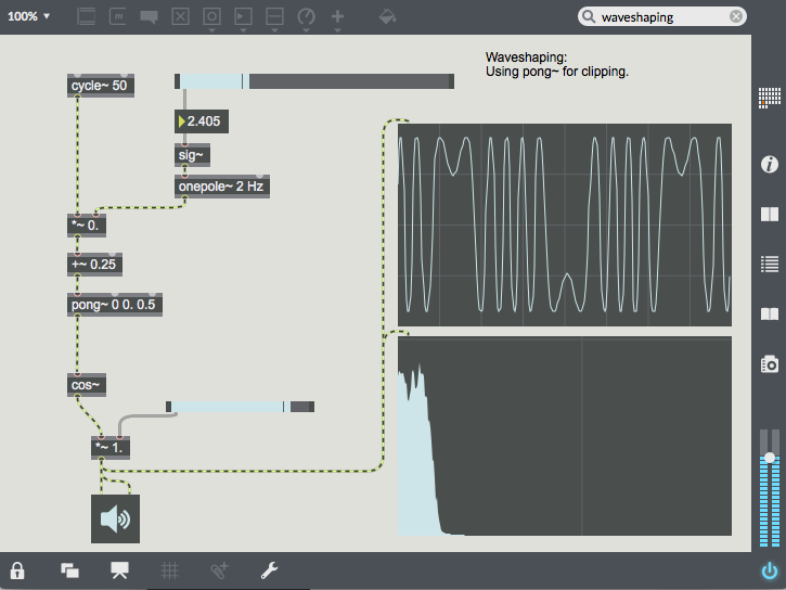
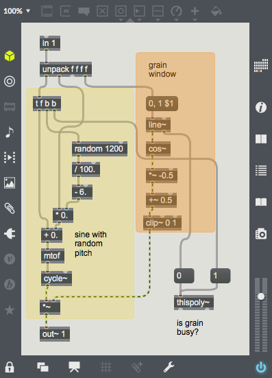
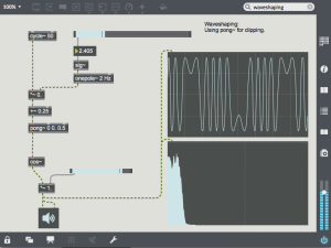 Another interesting type of wave shaping using half of a cos~ function and the wrap mode (0) of pong~. As the amplitude increases, the sin wave is reshaped through more and more cycles of a cosine function, resulting is a large number of new harmonics. This type of waveshping sounds much like FM synthesis (covered in next week’s lesson).
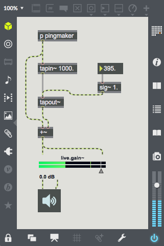 Delay is a method of transmitting sound through a media so that it can be heard later. This media can be magnetic tape, digital memory, or even the air.
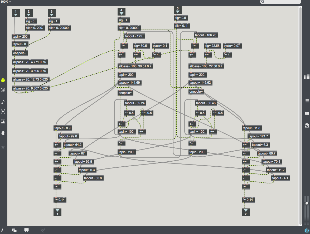
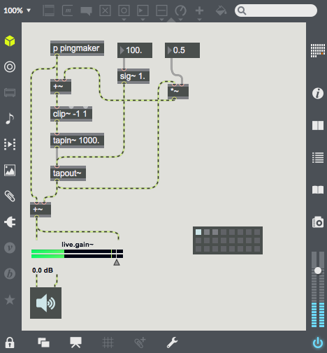 With many natural acoustic spaces (e.g. in a large room), the delayed sound re-enters the delay after it is heard, and the echo is repeated many times. This repeat can be easily added by sending some of the sound from tapout~ back into tapin~. In this patch, the output is multiplied by a feedback gain of 0.5 and added to the input signal before entering the delay line. This gain represents the gain reduction after each echo. If you select the first preset, you will here multiple decaying echoes. The second preset has much less gain reduction, and is an example of a rhythmic use of delay. The third preset shows the effect of having gain at or above 1.0. The signal soon clips and the delay memory soon fills with distortion. The clip~ object is essential to prevent the volume from getting out of control.
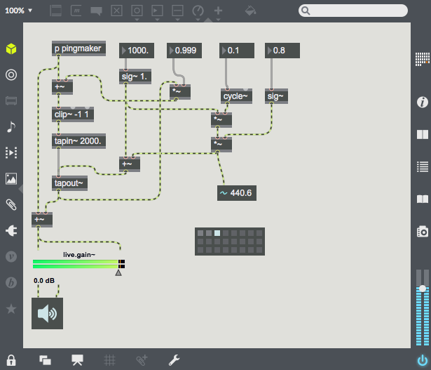 This next patch shows the simple addition of a sine oscillator as a modulation source for the delay time. When time is modulated, the period of any pitched material in the delay line is expanded and contracted. This will cause doppler pitch shifting effects. The 4 presets show various types of time modulation. The fourth example uses an audio frequency modulation oscillator. This will frequency modulate the contents of the delay memory. Flange, chorus and pitch shifting are all created using carefully tuned time modulation. Try to expand on this patch to create these effects. It will help to use sound sources other than the percussive “pingmaker” subpatch to demonstrate these effects.